5.12 Multilevel analysis

Through the command regress-mml you can perform multilevel analyzes with up to three levels. This type of analysis allows you to check relationships related to both individual and group-related characteristics.

Multilevel analyses, also known as hierarchical linear models or mixed effects models, are a type of statistical analysis that takes into account natural hierarchy or grouping in the data. For example, students (level 1) may be grouped into classes (level 2), which in turn are grouped into schools (level 3). Multilevel analyzes allow you to examine how variables at different levels affect the outcome variable, and how effects may vary between groups.

While standard linear regression models (OLS) allow you to analyze the effect of individual characteristics on an outcome variable, through multilevel analyzes you can also study effects linked to group characteristics. Multilevel analyzes can be seen as an advanced version of OLS in that one can study data organized at more than one level.

When choosing group variables in a multilevel analysis, it is important to think about the following:

• Theoretical understanding: The group variable should be meaningful in relation to what you are going to analyse

• Hierarchy: The group variables should have a hierarchical structure. For example, one can analyze students (level 1) who are grouped in schools (level 2) which are in turn grouped in districts (level 3).

• Variation between and within groups: There should be sufficient variation both between the groups (to be able to estimate group effects) and within the groups (to be able to estimate individual effects).

• Group size: The groups should not be too small, because this can make it difficult to reliably estimate group effects. There should be enough observations within each group to provide reliable estimates.

• Avoid overlap between groups: If there is overlap between groups (for example, if individuals may be members of multiple groups), it may be more appropriate to model them as crossed effects rather than nested effects. The command regress-mml currently does not allow crossed effects.

To investigate whether a categorical variable is suitable as a group variable, you can use the commands boxplot or histogram. You use the outcome variable as an argument, and the group variable to group the display. Example:

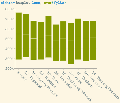Boxplot diagram that gives an insight into how the wage spread looks for each of the counties. This is a way of checking whether county is a good choice as a group variable. The more the spread and mean/median varies for the different group values, the better. Then the group variable will most likely explain part of the total variance. You can also create histograms that are grouped by county (histogram wage, by(county)). This gives a more thorough insight into the distribution of wages by county.

The regress command allows you to run a standard linear regression. In practice, this is a one-level model that can act as a reference for the estimates you get when you run multilevel analyzes through the regress-mml command. Example:

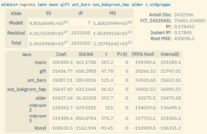Population: Permanent residents at the end of 2022, aged 20-60. Ordinary linear regression: Effect of gender, marital status married, number of children, social background (at least one of the parents has higher education), age and level of education (1-3 where 3 is the highest) on wage. Values ​​apply to 2022.

Multilevel analyzes can be run in almost the same way as for regression. Instead, you run the command regress-mml where you enter the group variable after a by clause in the model expression. Example of a two-level model where county of residence constitutes level two:

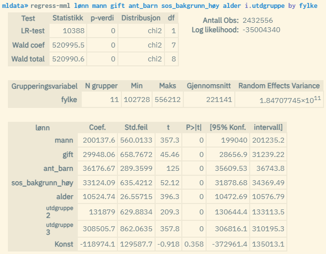Same population and variables as in the example above. But here a two-level analysis is used where the analysis units are grouped by county of residence. The contribution from county membership is estimated here in addition to the personal characteristics given by the explanatory variables.

By entering two group variables, a three-level model can be run. This is the highest level allowed. Remember that the group variable that defines the highest hierarchy level must be entered first. Example where you use education level and hierarchical occupational group as respectively level 3 and 2:

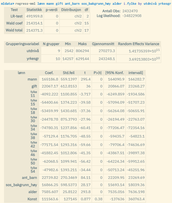Same population and variables as in the example above. In addition, county of residence is used here as an explanatory variable. Here, a three-level analysis is used where the analysis units are grouped by education level (0-8 where 8 is the highest) and hierarchically divided occupational group (0-9 where 0 is unspecified and military occupations, 1 is the highest (management occupations), and 9 is the lowest (occupations without education requirements)). Here, the contribution from belonging to a group is estimated based on education level and occupational categorization in addition to the personal characteristics given by the explanatory variables. Education level is level 3, and occupational group is level 2.

Explanation to the results:

• Antall Obs: Total number of units (usually people) used in the analysis (N)

• Log Likelihood: Log Likelihood value based on Restricted/Residual Maximum Likelihood estimation. Gives a measure of how well the model fits the data (often shows negative values, and the higher the number (less negative) the better the model)

• LR-test: Test for explanatory power in relation to a standard OLS estimation without group variables (the higher the statistical value, the better). p-value < 0.05 means that the multilevel model provides a significantly better explanation of total variance. df = number of degrees of freedom = number of group variables (max 2)

• Wald coef: Wald test for the explanatory power of the explanatory variables (the higher the statistical value, the better). p-value < 0.05 means that the overall effect of the explanatory variables is significantly different from 0. df = number of degrees of freedom = number of explanatory variables

• Wald total: Wald test where the group variables are also included in the test.

• N grupper: Number of groups for each group variable

• Min: Minimum number of group units for each group variable

• Maks: Highest number of group units for each group variable

• Gjennomsnitt: Average number of units in each group, for each group variable

• Random Effects Variance: Overall measure of the variance of the dependent variable for each level represented by the group variables. The higher the value, the greater part of the total variance can be explained by the group variables. The value can be seen in connection with the SS values ​​for the total model (Total Sum of Squares) which are reported through normal OLS analysis (run regress with the same variable set-up minus group variables). This gives an estimate of how much of the total variance can be attributed to group effects.

 $\rhd$ Practical examples: Script for recreating the analyzes referred to in the examples above

Source:

The algorithms for the command regress-mml are based on the regression class mixedlm in the Python package statsmodels: https://www.statsmodels.org/devel/generated/statsmodels.regression.mixed_linear_model.MixedLM.html